With the start of CBB season last week, the SB Nation blog covering Mid-Majors (Mid-Major Madness) introduced a new fantasy game, Mid-Major Stock Exchange. The premise, similar to the stock market, is to create a portfolio with $500.
I’ll be honest, I don’t watch a lot of mid-major basketball. Mostly just nationally televised games and the Aggies. This seemed like a prime chance to flex Linear and Integer Programming. Linear and Integer Programming is used in many industries to focus on resource allocation, the goal is to find optimal solutions.
In my case, I wanted to optimize returns on mid-major teams. Here is where I encountered the first problem, this is the pre-season and we have not had any games (or previous history in this game) to identify returns. However, if I can correlate team rankings (created from analytics methods) with the cost set it’s possible to estimate potential returns.
Team Ranking-Cost Correlations
If anyone’s interested, I’d definitely look at @brian_lefevre1 work. I used a variation of his pre-season ranking system. First let’s take a look at how the rankings compare to the cost set.
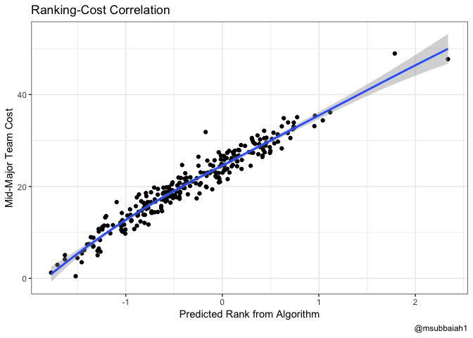
The rankings and the cost are similar enough, that I’m confident with using the standard errors of the team rankings as part of a random walk to estimate the cost in the future. The team rankings are derived from a linear regression, estimating the adjusted efficiency margins.
Estimating Future Costs
Random Walk forecasting looks something like this:
\[\begin{align*} y\_{1} = y\_{0} + e\_t \\ y_{1} = y_{0} + e_t \end{align*}\]
In our case, cost will be estimated as follows
\[\begin{align*} C_{1} = C_{0} (1+\mathcal{N}(\mu,\sigma)) \\ C_{2} = C_{1} (1+\mathcal{N}(\mu,\sigma)) \end{align*}\]
The rowwise function in dplyr is key here, otherwise we would use the same random number to estimate future costs for these teams. Later when determining the returns, the differences would all be the same.
There are a few teams that have just joined the D-1 ranks or for some reason data is missing. For this, I imputed values based on similar teams. Similarity was defined by teams who had a similar cost (within a 5% margin). The code for this can be seen below.
ecdf_fun <- function(x,perc) ecdf(x)(perc)
impute_values <- function(df){
  inds <- which(is.na(df$predTeamRk))
  for(val in inds){
    cost_search <- df[val,'Cost'] %>% pull()
    percent_val <- ecdf_fun(sort(df$Cost),cost_search)
    top_pct <- percent_val + 0.05
    low_pct <- percent_val - 0.05
    range_val <- quantile(df$Cost, probs = c(low_pct, top_pct))
    search_df <- df %>% filter(Cost >= range_val[1] & Cost <= range_val[2]) %>% drop_na()
    median_val <- median(search_df$predTeamRk)
    df[val,"predTeamRk"] <- median_val
  }
  return(df)
}


combine_df <- impute_values(combine_df)set.seed(41)
combine_df <- combine_df %>% rowwise() %>%
mutate(
ret = Cost * (1+rnorm(1,mean=0,sd=se.val)),
ret2 = ret * (1+rnorm(1,mean=0,sd=se.val)),
ret3 = ret2 * (1+rnorm(1,mean=0,sd=se.val)),
ret4 = ret3 * (1+rnorm(1,mean=0,sd=se.val)),
ret5 = ret4 * (1+rnorm(1,mean=0,sd=se.val)),
ret6 = ret5 * (1+rnorm(1,mean=0,sd=se.val)),
ret7 = ret6 * (1+rnorm(1,mean=0,sd=se.val)),
ret8 = ret7 * (1+rnorm(1,mean=0,sd=se.val)),
ret9 = ret8 * (1+rnorm(1,mean=0,sd=se.val))
)Now to calculate the returns, we take the difference of the cost matrix.
##      abilene christian air force    akron
## [1,]          17.81000  20.49000 23.08000
## [2,]          17.56942  20.54356 23.47112
## [3,]          17.59705  20.57641 23.09482
Here is a snapshot of the return matrix. The median of the returns matrix is used as the main objective function in the integer program.
##      abilene christian    air force        akron
## [1,]      -0.013508198  0.002614065  0.016946222
## [2,]       0.001572699  0.001598822 -0.016032414
## [3,]      -0.015698671 -0.001535754 -0.008860428
Linear/Integer Programming
Finally to the good stuff. How do I go about allocating which teams to submit in my portfolio. Linear programs focus on maximizing or minimizing an objective function with a set of constraints. It solves for optimal values of the variables such that the objective function is maximized, in this case.
The objective function here is to be maximized based on the estimated median returns found earlier. The first constraint is to ensure that the total of the investments (all stocks purchased) should amass to less than or equal to $500. Another common constraint is ensuring that the values (stocks) are integers.
Additionally, I added in another constraint to ensure that no more than 10 shares were owned of each team. Since the matrix was a tad large, the lpSolveAPI package is much more robust than lpSolve.
Here we set up the IP, and provide the names of all the teams such that the output is much easier to read.
library(lpSolveAPI)
n = length(ret_mat2)
fund_allocate <- make.lp(0,n)
yNames <- names(ret_mat2)
colnames(fund_allocate) <- c(yNames)
Objective
Here we set the objective
set.objfn(fund_allocate,c(matrix(ret_mat2, ncol=1, byrow=TRUE)))Constraints
Now come the constraints
costs <- combine_df %>% pull(Cost)
add.constraint(fund_allocate,costs,"<=",500)
for(i in 1:n){
  add.constraint(fund_allocate,1,"<=",10,c(i))
}
lp.control(fund_allocate,sense='max')
set.type(fund_allocate, 1:ncol(fund_allocate), type = 'integer')
write.lp(fund_allocate,'funds.lp',type = 'lp')
Not to add a few final touches. Ensuring that the objective function is maximized (we don’t want to minimize our returns…..) and to treat this as an integer program (only whole stocks).
I ended up submitting two portfolios, I made a mistake in my coding, happens to everyone. I accidentally left the problem type set to binary. It was kind of a nice mistake because this allowed me to see what a more diverse portfolio would be if I only invested in each team once.
A final note I wrote the LP to a text file. It’s helpful to go back and check the text file because the linear program is written out in a clean format.
Results
Here is the suggestion on who to invest in for my main portfolio.
status = solve(fund_allocate)
print(get.objective(fund_allocate))
[1] 9.554434
solution = get.variables(fund_allocate)

names <- yNames[which(solution!=0)]
shares <- solution[which(solution!=0)]
cost <- costs[which(solution!=0)]

cost_df <- data.frame(Team=names,Shares=shares,Cost=cost)
cost_df <- cost_df %>% mutate(total_cost = cost*shares)
cost_df %>% kable(format="markdown")| Team | Shares | Cost | total_cost |
|---|---|---|---|
| delaware state | 9 | 1.25 | 11.25 |
| drake | 3 | 19.82 | 59.46 |
| florida atlantic | 10 | 13.56 | 135.60 |
| nevada | 6 | 48.94 | 293.64 |
Here is the suggestion on who to invest in for my diverse portfolio.
| Team | Shares | Cost | total_cost |
|---|---|---|---|
| arkansas pine bluff | 1 | 7.07 | 7.07 |
| byu | 1 | 36.14 | 36.14 |
| delaware state | 1 | 1.25 | 1.25 |
| drake | 1 | 19.82 | 19.82 |
| florida atlantic | 1 | 13.56 | 13.56 |
| florida gulf coast | 1 | 21.01 | 21.01 |
| grand canyon | 1 | 25.57 | 25.57 |
| incarnate word | 1 | 7.46 | 7.46 |
| jacksonville | 1 | 15.36 | 15.36 |
| middle tennessee state | 1 | 25.63 | 25.63 |
| missouri state | 1 | 21.90 | 21.90 |
| murray state | 1 | 27.50 | 27.50 |
| nevada | 1 | 48.94 | 48.94 |
| north dakota state | 1 | 20.69 | 20.69 |
| north texas | 1 | 24.50 | 24.50 |
| oral roberts | 1 | 18.79 | 18.79 |
| prairie view a&m | 1 | 13.65 | 13.65 |
| st peters | 1 | 21.94 | 21.94 |
| st francis pa | 1 | 24.36 | 24.36 |
| umbc | 1 | 18.91 | 18.91 |
| usc upstate | 1 | 10.74 | 10.74 |
| texas san antonio | 1 | 24.48 | 24.48 |
| vcu | 1 | 27.77 | 27.77 |
| wagner | 1 | 21.71 | 21.71 |
Full code can be found here.